1. Trashcan selection
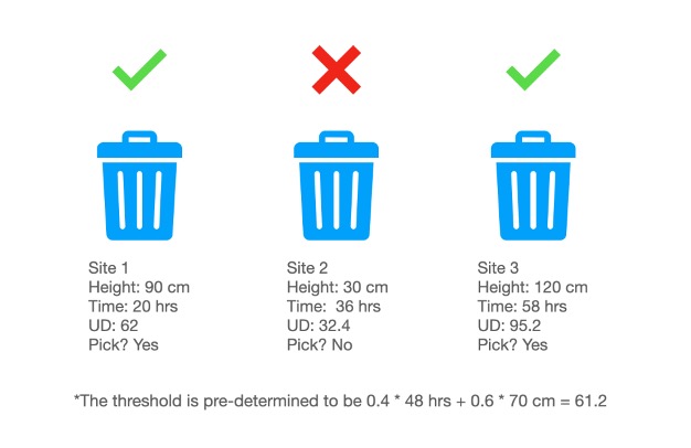
In order to further reduce fuel consumption, I can first determine the exigency of a can to be picked as the first thing the program does every day before moving on to running algorithm. As a result, the driver does not need to visit every trashcan every day, if certain cans are not so urgent to be processed. To this end, I use the data recorded by detection sensors to calculate what is called urgency degree to determine the necessity of a bin to be processed today. Then comes to calculation of urgency degree: if it exceeds a predetermined threshold, I mark the can as necessary to be processed today, otherwise don't and leave it until the next day's examination comes. The urgency degree is calculated using equation below:
Figure 7 demonstrates 3 trashcans' necessity of being picked up today with premise that the threshold is 61.2. Therefore, the overall process in this step can be summarized in the flowchart below.

2. Route selection
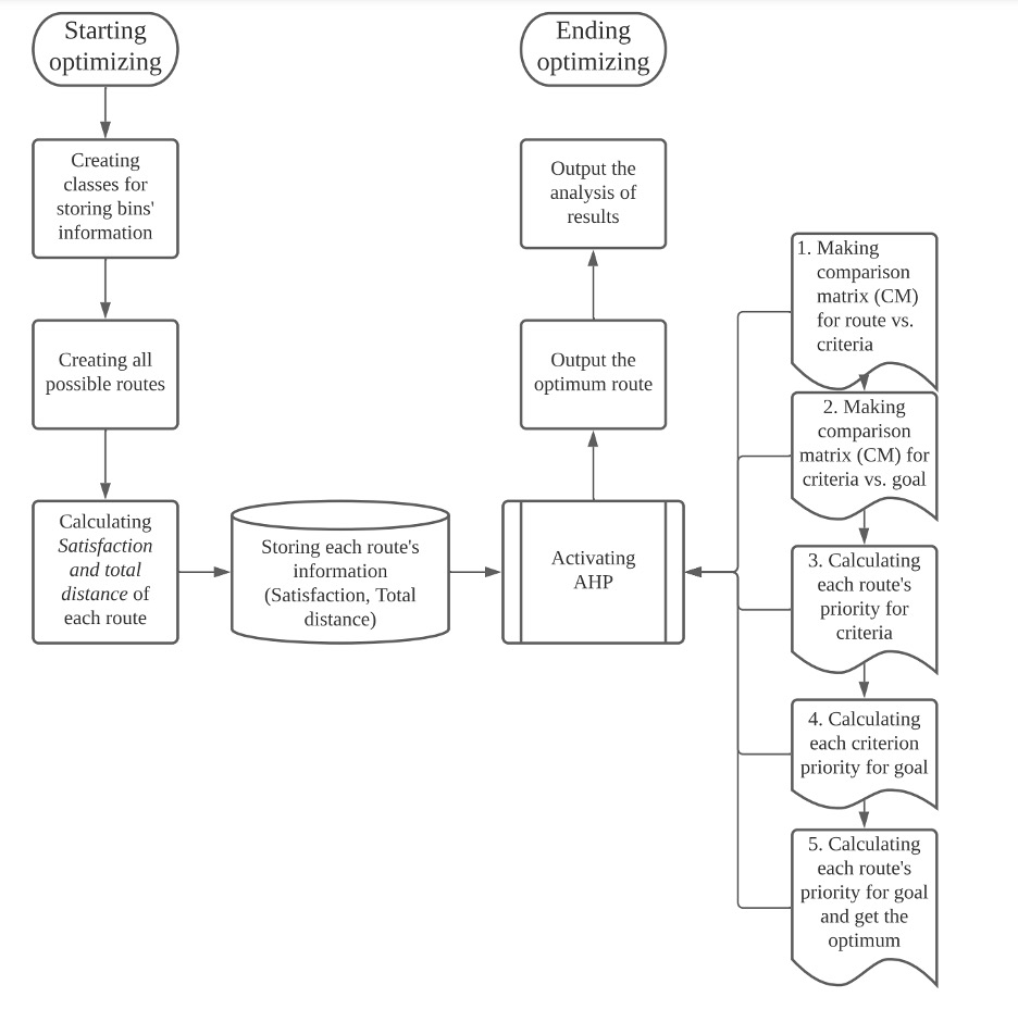
Generally, in singling out the optimal route, there are 7 steps involved: 1) creating classes for storing bins' information; 2) creating all possible routes; 3) calculating satisfaction and total distance of each route; 4) storing each
route's information in another class; 5) running AHP; 6) output the optimal route; 7) output the analysis of results. The flowchart describing the overall process is demonstrated in figure 8.

2.1 Producing the initial pool
After knowing trashcans necessary to be processed today, I then have to generate the pool, or all possible routes starting from one trashcan, travelling through all other trashcans, to the final one.
Since it is assumed that every two cans have at least one path connecting, I can say every can is connected to all the other ones. As such, permutation is most suitable for producing the pool. For instance, in the case of dealing with 5
waste bins, I can create a list that stores the sequence of visit; namely, [1, 2, 3, 5, 4] means starting from site 1, I sequentially go to site 2, 3, 5, and eventually 4. Thus, I just need to produce all, conclusive variants of this list
so that I can have a complete pool of candidates (for now).

2.2 Completing the pool
Now, holding the pool, I need to create variants further, since every two cans may have more than just one path. Hence, if, say, I are creating variants for a particular sequence list [1, 2, 3, 4, 5], where site 2 and 3 have 3 paths between them, then I can create in total of 3 variants for this sequence list. These variants differ from the original one in total travelled distance, which is one of the factors I consider when deciding the optimal route. I add new variants created from this process to the initial pool. At this point, the pool is completely conclusive and ready for the next step.
2.3 Forming new factor
It is inappropriate to directly take time and height as criteria, since what I are comparing is routes. So, when comparing 2 routes, there is no meaning to compare their time and height. Instead, I can combine the two factors into one more suitable acting as a criterion--Satisfaction. Specifically, in dealing with the case, and the case only, of determining sequence of trashcan to be processed, I know, in fact, the best sequence in the first place when detection sensors record each can's information. Clearly, I want trashcans that are most urgent to get processed to be prioritized, so I can create a standard model according to this fact, where the model is the best sequence starting from the most urgent trashcan to the least. Then, I evaluate the difference between the standard model with each of the routes in the pool. The more they are alike, the higher the satisfaction is.
2.4 Running AHP
Now I have two criteria when determining the optimal route: satisfaction and total distance.
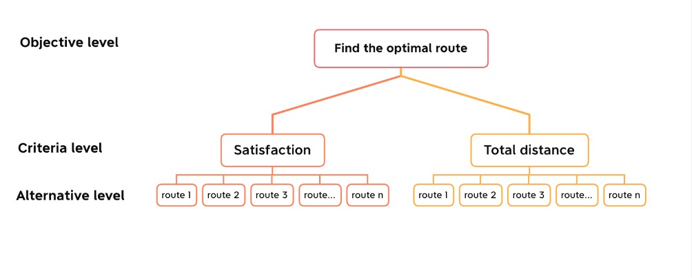
Since our goal is to single out the optimal route among the pool, this is a decision problem. I can construct the problem on 3 levels: objective, criterion, alternative. Therefore, in short, our goal is to determine the best alternative
considering all criteria that best meet the objective, as can be shown from figure 9 below.


2.5 Analysis of results
Calculation of fuel consumption
The average fuel consumption by pickup truck, in meters per liter, is 2.8 mpg, or 1190.4 meters per liter (APTA, 2019). So, I can divide the total distance of a route by this average to get average fuel consumption during this route.

CO2 emission is gained by multiplying the total liters of fuel burned during the route by the average CO2 in one liter. The average CO2 emission per gallon of gasoline is 2347.697 grams (Statista, accessed: Sep 7, 2021).

Notes about China's residential abodes
Note, the apartments in China is estimated to 6.45 millions (EPA, accessed: Sep 7, 2021) and I divide it by 5 since I are taking 5 apartments at a time to analyze optimal route amongst them.
2.6 Example of algorithm running in real case
I use an example to illustrate the whole process described above. First of all, I chose 5 apartments, JY, YG, BJ, JK, MW in my district, measured the distance between each two of them, and stored them into a chart.

